The theoretical prediction that did not fit a wrong experimental finding and was probably right

The superluminal group velocity difference of neutrinos that was NOT measured by Opera

I take advantage of the Physics Nobel Prize 2015 rewarding the discovery of neutrino oscillations to shine a different light on a famous experiment that made big headlines in september 2011 (and gave me opportunity to start this blog!)

we discuss the possibility that the apparent superluminality is a quantum interference effect, that can be interpreted as a weak measurement [2, 3, 4, 5]. Although the available numbers strongly indicate that this explanation is not correct, we consider the idea worth exploring and reporting – also because it might suggest interesting experiments, for example on electron neutrinos, about which relatively little is known. Similar suggestions, though not interpreted as a weak measurement [6, 7] or not accompanied by numerical estimates [6, 8], have been proposed independently. 

The idea, following analogous theory and experiment [9] involving light in a birefringent optical fibre, is based on the fact that the vacuum is birefringent for neutrinos. We consider the initial choice of neutrino flavour as a preselected polarization state, together with a spatially localized initial wavepacket. Since a given flavour is a superposition of mass eigenstates, which travel at different speeds, the polarization state will change during propagation, evolving into a superposition of flavours. The detection procedure postselects a polarization state, and this distorts the wavepacket and can shift its centre of mass from that expected from the mean of the neutrino velocities corresponding to the different masses. This shift can be large enough to correspond to an apparent superluminal velocity (though not one that violates relativistic causality: it cannot be employed to send signals). Large shifts, corresponding to states arriving at the detector that are nearly orthogonal to the polarization being detected, are precisely of the type considered in weak measurement theory. 

It seems that only muon and tau neutrino flavours are involved in the experiment... The initial beam, with ultrarelativistic central momentum p, is almost pure muon, which can be represented as a superposition, with mixing angle θ, of mass states |+> and |- >, with m₊ > m_- ... The two mass states evolve with different phases and group velocities neglecting the spreading and distortion [10] of the individual packets – both negligible in the present case. E_± and v_± are the energies and group velocities of the two mass states, and we write E_±=E±1/2ΔE, v_±=v±1/2Δv, x=vt+ξ... in which the new coordinate ξ measures deviation from the centre of the wavepacket expected by assuming it travels with the mean velocity. In the experiment, the detector postselects the muon flavour [1]... thus the shift in the measured final position of the wavepacket [can be interpreted]... as an effective velocity shift, that is  

[where the prefactor, tΔv is the relative shift of the two mass wavepackets, expected from the difference of their group velocities (it is small compared with the width of the packet ... in the neutrino case). The main factor represents the influence of the measurement-that is of the pre- and postselection and the evolution]... The possibility of superluminal velocity measurement arises because the amplification factor in (8) can be arbitrarily large if sin²2θ and sin²(tΔE/2ℏ) are close to unity, corresponding to near-orthogonality of |pre> and |post>. 

For neutrinos with momentum p, ... the group velocity [difference Δv is given by -ΔE/p]. Thus Δv<0, so, in order for the apparent velocity to be superluminal, Δveff in (8) must be positive; this can be accommodated by making cos2θ negative. 

Note also that v₊ and v_-- are less than c if both neutrino masses are nonzero, so the individual mass eigenstate wavepackets move with subluminal group velocities; any superluminal velocity arising from (8) is a consequence of pulse distortion ... associated with the postselection, i.e. considering only arriving muon neutrinos. In the more conventional superluminal wave scenario [10], group velocities faster than light, and the pulse distortions that enable them to occur, are associated with propagation of frequencies near resonance, for which there is absorption, i.e. non-unitary propagation. That is also true in the optical polarization experiments [9] and in the neutrino situation considered here, with the difference that the nonunitarity, which gives rise to the superluminal velocity, is not continuous during propagation but arises from the sudden projection onto the postselected state.

In the [Opera] experiment, the energies of the neutrinos varied over a wide range, with an average of cp = 28.1GeV. For the difference in the squared masses, with electron neutrinos neglected and m₊ and m_- identified with the standard m₂ and m₃, a measured value [13] is m₊²c⁴-m_-²c⁴≃2.43×10^-3eV². This gives

Δv/c=-1.5×10^-24.                  (16) 

 The apparent velocity measured in the experiment [1] was (1+2.5×10^-5)c . Comparison with the quantum velocity shift Δv_eff in (8) would require knowlege of m₊ and m_-, not just their squared difference, and the individual masses are not known. But even on the most optimistic assumption, that m_-=0, it is immediately clear that it is unrealistic to imagine that the quantum amplification factor in (8) can bridge the gap of 19 orders of magnitude between (16) and the measured superluminal velocity.

Can apparent superluminal neutrino speeds be explained as a quantum weak measurement?

M. V. Berry, N. Brunner, S. Popescu, P. Shukla

(Submitted on 13 Oct 2011 (v1), last revised 14 Nov 2011 (this version, v2))

Remark: for the anecdote the abstract of this article by the distinguished mathematical physicist Michael Berry and his collaborators might be the shortest one ever written since it answered laconically to the question asked in the title : "probably not". And time has proved that it was right...

A superluminal group velocity of photons that was effectively measured
While the theoretical prediction from the last paragraph has not been tested by the Opera experiment and will stay quite hard to test empirically given the smallness of the effect, the physics behind it is pretty sound and falsifiable in other contexts. I think the article below is a nice illustration:

The physics of light propagation is a very timely topic because of its relevance for both classical [1] and quantum [2] communication. Two kind of velocities are usually introduced to describe the propagation of a wave in a medium with dispersion ω( k): the phase velocity v_ph=ωk and the group velocity v_g=∂ω/∂k . Both of these velocities can exceed the speed of light in vacuum c in suitable cases [3]; hence, neither can describe the speed at which the information carried by a pulse propagates in the medium. Indeed, since the seminal work of Sommerfeld, extended and completed by Brillouin [4], it is known that information travels at the signal velocity, defined as the speed of the front of a square pulse. This velocity cannot exceed c [5]. The fact that no modification of the group velocity can increase the speed at which information is transmitted has been directly demonstrated in a recent experiment [6]. Superluminal (or even negative) and, on the other extreme, exceedingly small group velocities, have been observed in several media [7]. In this letter we report observation of both superluminal and delayed pulse propagation in a tabletop experiment that involves only a highly birefringent optical fiber and other standard telecom devices. 

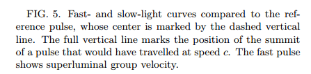
Before describing our setup, it is useful to understand in some more detail the mechanism through which anomalous group velocities can be obtained. For a light pulse sharply peaked in frequency, the speed of the center-of-mass is the group velocity v_g of the medium for the central frequency [3]. In the absence of anomalous light propagation, the local refractive index of the medium is n_f , supposed independent on frequency for the region of interest. The free propagation simply yields v_g=L/t_f where L is the length of the medium and t_f =n_f L/c is the free propagation time. One way to allow fast- and slow-light amounts to modify the properties of the medium in such a way that it becomes opaque for all but the fastest (slowest) frequency components. The center-of-mass of the outgoing pulse appears then at a time t = t_f+<t>, with <t> the mean time of arrival once the free propagation has been subtracted; obviously <t><0 for fast-light, <t>>0 for slow-light. If the deformation of the pulse is weak, the group velocity is still the speed of the center-of-mass, now given by  

                          v_g=Lt_f+<t>.                                                                         (1) 

This can become either very large and even negative (<t>→−∞) or very small (<t>→∞) — although in these limiting situations the pulse is usually strongly distorted, so that our reasoning breaks down.

 

Direct measurement of superluminal group velocity and of signal velocity in an optical fiber 

Nicolas Brunner, Valerio Scarani, Mark Wegmuller, Matthieu Legre, Nicolas Gisin

(Submitted on 20 Jul 2004 (v1), last revised 10 Jan 2005 (this version, v2))

Neutrino oscillations : experiment validated and awarded the 2015 Physics Nobel Prize ...

... but theory is still under [discuss]{construct}ion

Neutrino physics is one of the most interesting and vividly discussed topics in high-energy physics today. Especially the question whether the neutrinos can oscillate or not (i.e. different neutrinos can change into each other) gave rise to a huge number of experiments to actually observe these oscillations. At least since the results from the Super Kamiokande ... and the SNO experiment ... are published, it is widely believed that neutrino oscillations are an experimentally verified fact. However, the first hint has already been found in 1964 when the Homestake experiment ... discovered the solar neutrino problem. That is, the number of measured electron neutrinos from the sun is by a factor of 2-3 less than the number of neutrinos predicted by the standard solar model (SSM). 

Since within the standard model (SM) of particle physics the neutrinos are massless, and consequently cannot oscillate, their measurement shows that new physics beyond the SM exists. And indeed nowadays the experiments on neutrino oscillations are important to measure the unknown parameters of the SM and its minimal extensions. In particular, these unknown parameters are the neutrino masses and the entries in the neutrino mixing matrix. 

From all the measurements made to discover neutrino oscillations one should think that the theory behind [them] is well established and understood. But surprisingly this is not the case. The first who mentioned the idea of neutrino oscillations, though he assumed neutrino-antineutrino oscillations, was Pontecorvo in 1957 [Pon57, Pon58]. A few years later Maki, Nakagawa and Saka were the first to consider oscillations between the electron and the muon neutrino [MNS62]. Then it took around 20 years before Kayser in 1981 showed that the up to that point used plane-wave approximation cannot hold for oscillating neutrinos and he proposed a wave packet treatment [Kay81], which then has again not been discussed for around 10 years. In the early 90s the discussion on the theoretical description of neutrino oscillations finally started with several seminal papers. First, Giunti, Kim and Lee explicitly calculated the oscillation probability for the neutrinos in a wave packet model [GKL91] and then showed that the state vectors used for the quantum mechanical description are, in general, ill-defined [GKL92]. In 1993 they published together with Lee a calculation of the probability in a quantum field theoretical framework without using state vectors for the neutrinos [GKLL93]. And finally, in 1995 Blasone and Vitiello showed that the description of mixed particles in quantum field theory (QFT) yields unexpected problems for the interpretation of neutrinos as particles. By only using exact—without perturbation—QFT methods they calculated an oscillation probability which differs significantly from the other results [BV95]. All these different approaches are even today still under discussion, but however under the assumption of relativistic neutrinos which have tiny mass squared differences, all approaches give the same result. Thus, the theoretical discussion on the right description of the neutrinos does not spoil the experimental results, because today we are only able to measure ultra-relativistic neutrinos whose energy is at least a few orders of magnitude higher than their mass. 

Diploma Thesis On Theories of Neutrino Oscillations (Summary and Characterisation of the Problematic Aspects) Daniel Kruppke September 2007

A quantum field theory for flavor states ...

The study of mixing of fields of different masses in the context of Quantum Field Theory (QFT) has produced recently very interesting and in some sense unexpected results ... The story begins in 1995 when in Ref.[1], it was proved the unitary inequivalence of the Hilbert spaces for (fermion) fields with definite flavor on one side and those (free fields) with definite mass, on the other. The proof was then generalized to any number of fermion generations [7] and to bosonic fields [2, 5]. This result strikes with the common sense of Quantum Mechanics (QM), where one has only one Hilbert space at hand: the inconsistencies that arise there have generated much controversy and it was also claimed that it is impossible to construct an Hilbert space for flavor states [16] (see however Ref.[6] for a criticism of that argument). In fact, not only the flavor Hilbert space can be consistently defined [1], but it also provide a tool for the calculation of flavor oscillation formulas in QFT ..., which exhibit corrections with respect to the usual QM ones [20, 21]. From a more general point of view, the above results show that mixing is an “example of non-perturbative physics which can be exactly solved”, as stated in Ref.[13]. Indeed, the flavor Hilbert space is a space for particles which are not on-shell and this situation is analogous to that one encounters when quantizing fields at finite temperature [22] or in a curved background [23]. In the derivation of the oscillation formulas by use of the flavor Hilbert space, both for bosons and for fermions, a central role is played by the flavor charges [9] and indeed it was found that these operators satisfy very specific physical requirements [6, 8]. 

Mixing and oscillations of neutral particles in Quantum Field Theory

Massimo Blasone, Jonathan S. Palmer

(Submitted on 23 May 2003 (v1), last revised 10 Jun 2003 (this version, v2))

... with an unfinished taste

Blasone and Vitiello (BV) have attempted to construct a Fock space for neutrino flavor states [4]... Giunti conclude that “the Fock spaces of flavor neutrinos are ingenuous mathematical constructs without physical relevance” [3]. 

... there is another issue that plagues the scheme in [5]. The problem is that the neutrino flavor vacuum defined in [5] is time-dependent and hence Lorentz invariance is manifestly broken. Recently, BV and collaborators attempted to tackle this issue by proposing neutrino mixing as a consequence of neutrino interactions with an external non-abelian gauge field [7]. Under this framework, the Lorentz violation of the neutrino flavor vacuum can be attributed to the presence of a fixed external field which specifies a preferred direction in spacetime. However, at the moment, there is not a single sign of such a non-abelian gauge field in neutrino experiments. They proposed that this scheme can be tested in the tritium decay, but again the indefinite mass mνα becomes an observable quantity. Also, given the current stringent bounds on Lorentz violations [8], it is unclear whether this scheme will survive... 

In this article, we first gave a detailed review on the current status of the understanding about the neutrino flavor states. At the end of the review, we were led to conclude that it is currently unclear how to construct a consistent and physically relevant Fock space of neutrino flavor states. We proceeded to prove that if one insists on second-quantizing the neutrino flavor fields and thereby constructing the flavor states, then they are approximately well-defined only when neutrinos are ultra-relativistic or the mass differences are negligible compared to energy...   

However, we showed that one can consistently describe weak interactions by only neutrino mass eigenstates. At the same time, we argued that the second quantization of neutrino flavor fields generally lacks physical relevance because their masses are indefinite. Thus, neutrino flavor states lose their physical significance and they should simply be interpreted as definitions to denote specific linear combinations of mass eigenstates involved in weak interactions. Under this interpretation, there is no physical motivation to construct the Fock space of neutrino flavor states from the first principles of quantum field theory. 

On Neutrino Flavor States

Chiu Man Ho

(Submitted on 16 Sep 2012 (v1), last revised 26 Nov 2012 (this version, v2))

My quantum ostinato : the standard model can not stay out of the revolution of spacetime

This short post aims at two things:

• to thank Jackson Clarke author of the very informative blog Syymmetries to put Transcyberphysix  in his recent list of "recommended (active) high energy physics news and blog links".

• to suggest to any internaut arrived here through the former blog links to visit Quantum Ostinato another blog of mine which is currently more active than this one and might bring piece of information less covered by other blogs but relevant for people interested in high energy physics and astrophysics. 

Two scalars to rule the m(ass for almost) all (particles)? / Deux scalaires pour gouverner (presque) toutes les masses

The advanced art of massware in electroweak and QCD quantum vacua/ L'art subtil de la génération de masse dans les vides quantiques électrofaibles et chromodynamiques
This post is a follow-up to this one. / Ce billet fait écho à celui-ci vieux de plus d'un an.

In the standard model the masses of elementary particles arise from the Higgs field acting on the originally massless particles. When applied to the visible matter of the universe this explanation remains unsatisfactory as long as we consider the vacuum as an empty space. The QCD vacuum contains a condensate of up and down quarks. Condensate means that the qq̅ pairs are correlated via inter-quark forces mediated by gluon exchanges. As part of the vacuum structure the qq̅ pairs have to be in a scalar-isoscalar configuration. This suggests that the vacuum condensate may be described in terms of a scalar-isoscalar particle, |σ>=(|uu̅>+|dd̅>)/√2, providing the σ field. These two descriptions in terms of a vacuum condensate or a σ field are essentially equivalent and are the bases of the Nambu–Jona-Lasinio (NJL) model [2–8] and the linear σ model (LσM), [9] respectively. Furthermore, it is possible write down a bosonized version of the NJL model where the vacuum condensate is replaced by the vacuum expectation value of the σ field. 

In the QCD vacuum the largest part of the mass M of an originally massless quark, up (u) or down (d), is generated independent of the presence of the Higgs field and amounts to M = 326 MeV [1]. The Higgs field only adds a small additional part to the total constituent-quark mass leading to m u = 331 MeV and m d = 335 MeV for the up and down quark, respectively [1]. These constituent quarks are the building blocks of the nucleon in a similar way as the nucleons are in case of nuclei. Quantitatively, we obtain the experimental masses of the nucleons after including a binding energy of 19.6 MeV and 20.5 MeV per constituent quark for the proton and neutron, respectively, again in analogy to the nuclear case where the binding energies are 2.83 MeV per nucleon for 31 H and 2.57 MeV per nucleon for ³He. 

In the present work we extend our previous [1] investigation by exploring in more detail the rules according to which the effects of electroweak (EW) and strong-interaction symmetry breaking combine in order to generate the masses of hadrons. As a test of the concept, the mass of the π meson is precisely predicted on an absolute scale. In the strange-quark sector the Higgs boson is responsible for about 1/3 of the constituent quark mass, so that effects of the interplay of the two components of mass generation become essential. Progress is made by taking into account the predicted second σ meson, σ′(1344) = |ss̅> [7]. It is found that the coupling constant of the s-quark coupling to the σ′ meson is larger than the corresponding quantity of the u and d quarks coupling to the σ meson by a factor of √2. This leads to a considerable increase of the constituent quark masses in the strange-quark sector in comparison with the ones in the non-strange sector already in the chiral limit, i.e. without the effects of the Higgs boson. There is an additional sizable increase of the mass generation mediated by the Higgs boson due to a∼24 times stronger coupling of the s quark to the Higgs boson in comparison to the u and d quarks. In addition to the progress made in [1] as described above this paper contains a History of the subject from Schwinger’s seminal work of 1957 [10] to the discovery of the Brout-Englert-Higgs (BEH) mechanism, with emphasis on the Nobel prize awarded to Nambu in 2008. This is the reason why paper [1] has been published as a supplement of the Nobel lectures of Englert [11] and Higgs [12]...

The masses of constituent quarks are composed of the masses M_q predicted for the chiral limit and the mass of the respective current quark m⁰_q provided by the Higgs boson (EW interaction) alone. For scalar mesons the sum of M_q and m⁰_q leads to a zero-order approximation for the constituent-quark mass m_q, but there are dynamical effects described by the NJL model which modify the simple relation m_q=M_q+m⁰_q  , except for the non-strange sector where this relation is a good approximation. Similar results are obtained for the octet baryons. A difference between the scalar mesons and the octet baryons is that that for scalar mesons binding energies do not play a rôle whereas they are of importance in case of octet baryons... 

Mass generation via the Higgs boson and the quark condensate of the QCD vacuum

Martin Schumacher

(Submitted on 1 Jun 2015)

Slava Mukhanov can stick to his guns

Rubrique : Curiositêtes (#2)
\\Ce billet a été révisé le 08/02/2015

How many time is history repeating ?

Slava Mukhanov, another old-school Russian physicist ... was one of the first to realise that inflation wouldn't just cause the universe to expand dramatically and to make it more homogeneous, it would also seed new fluctuations with a very small amplitude. These new, small, fluctuations arise from the stretching (and eventual amplification) of quantum fluctuations in the field driving inflation. This type of realisation was what took inflation from an interesting concept to a testable paradigm. With satellites like Planck those perturbations are now being ever more precisely examined. 

Mukhanov has a very different perspective to [Alexeï] Linde regarding what inflation can or cannot explain. To him the question of whether a theory is scientific or not comes down to one thing and one thing only: has it made unique a priori predictions that can then either be verified or used to rule out the theory? From that perspective his view is that inflation has only ever predicted one set of results and those are the predictions of the first, simplest models of inflation. He makes no distinction as to whether those models are well described by a quantum field theory model or not. 

[...] Muhkanov deserves credit for at the very least sticking religiously to his guns. He likes to show slides during talks like this that were written on overhead transparencies in the early 90's. This dates these slides to an era before the anisotropies in the CMB were discovered, before the late-time accelerated expansion was discovered and a time when the total observed mass in the universe was indicating that the curvature in the universe might be significant (i.e. in technical terms it would be "open"). These slides make a number of specific predictions for what inflation requires (by Mukhanov's definition of inflation).

• A flat universe (i.e. no curvature)
• Perturbations that had a Gaussian distribution
• Perturbations that were almost scale-invariant, but not quite (they would need to have a slightly larger amplitude at larger scales)
• Perturbations that were adiabatic (i.e. all the constituents of the universe were perturbed in the same way)
• A small, but not insignificant quantity of primordial gravitational waves

How many of these predictions have now been verified?

All but one.

The reason why Mukhanov deserves credit is that at two separate points in history at least one of these predictions has been in serious jeopardy. [...] when Mukhanov was first writing these predictions down, there seemed to be some evidence that the universe was open. At that time, some inflationary theorists (Linde amongst them) were trying to construct models of inflation that could generate an open universe. Mukhanov said in his talk that at this point of history he was considering leaving cosmology because he believed inflation could not survive as a predictive science if the universe was open. It turned out that those tentative hints of openness were actually the first evidence of the consequences of the accelerated expansion and that the universe is flat.  

Then, last decade the WMAP satellite was showing not insignificant evidence for a large degree of "non-Gaussianity" in the CMB. If that had been verified, Linde's inflation would have survived (after all it can explain anything), but Mukhanov would have pronounced inflation dead. Planck showed that WMAP's evidence was only a statistical fluctuation and that, to Planck's accuracy, there is no evidence for primordial non-Gaussianity.

Mukhanov's view of inflation seems to be surviving quite well.

There is that one missing piece though. These are primordial gravitational waves.

The universe as seen by Planck - Days Three and Four I

Posted by Shaun Hotchkiss April 8, 2013

(Having) Great expectations (but not too great)

Although primordial gravitational waves are not yet detected, the experimental confirmation of the flatness of the universe, adiabatic nature of nearly gaussian perturbations and the discovered (at 3,5 sigma level) logarithmic tilt of the spectrum unambiguously prove the quantum origin of the universe structure and the early cosmic acceleration. Needless to say that all these predictions, which were yet in conflict with observations about 15 years ago, are very nontrivial. Given that the quantum origin of the universe structure is experimentally confirmed, the precision measurements already now allow us to exclude many inflationary scenarios existing in the literature. Moreover, the improved accuracy of the determination of spectral index, the bound (or detection) on non-gaussianity and the bound (or possible future detection) on primordial gravitational waves will allow us to put further restrictions on the admissible inflationary scenarios. However, this seems will not help us too much in recovering the fundamental particle physics behind inflation. In fact, the observational data only allow us to measure only the effective equation of state and the rate of its change in a rather small interval of scales. Keeping in mind unavoidable experimental uncertainty, the effect of unknown physics right after inflation and degeneracy in the scenarios discussed above we perhaps will never be able to find out the microscopical theory of inflation without further very essential input from the particle physics. On the other hand, the remarkable property of the theory of quantum origin of the universe structure is that the gravity seems does not care too much about microscopic theory providing needed equation of state, and allows us to make experimentally verifiable predictions. 

Quantum Cosmological Perturbations: Predictions and Observations

Viatcheslav Mukhanov

(Submitted on 15 Mar 2013)

Working to avoid metaphysical problems

The Planck measurements have unambiguously confirmed the main predictions of the theory of quantum origin of the universe structure. Namely, the adiabatic nature and the Gaussian origin of primordial perturbations were established beyond any reasonable doubt. Even more amazing, more nontrivial infrared logarithmic tilt of the spectrum, first predicted in [2], was discovered at 6 sigma confidence level. The simplest way to amplify the quantum fluctuations is provided by the stage of inflation. Although nobody doubt the quantum origin of the primordial fluctuations, there are still claims in the literature that basically the same mechanism of amplification of quantum fluctuations can work also either in a bouncing universe on the stage of super slow contraction [18] or in conformal rolling scenario [19]. The generated spectra in the alternative theories are not the predictions of the theory, but rather postdictions which are constructed to be in agreement with observations. Nevertheless, this is not enough to rule out these possibilities at the level of a ”theorem”. Thus, at the moment the only robustly established experimental fact is the quantum origin of the universe structure with a little uncertainty left for the mechanism of amplification of quantum fluctuations. To firmly establish that namely inflation has provided us this mechanism one has to find the primordial gravitational waves the lower bound on which for the spectral index ns=0.96 corresponds to r about 0.003. According to [3, 4] one of the main motivations for looking the alternatives to inflation is the failure of predictability of so called ”postmodern inflationary paradigm”. Paradoxically this trouble seems to be due to the same successful quantum fluctuations with the red-tilted spectrum which lead to the galaxies. On one hand the quantum fluctuations explain the observed large scale structure of the universe, but on the other hand they are also responsible for the selfreproduction and produce eternal inflating multiverse where ”anything can happen and will happen an infinite number of times” [5]. In this paper I have shown how this problem can be avoided. Using the effective description of inflation I have found nearly unambiguous extension of inflation which avoids the selfreproduction. What is yet missing in this description is a justification of the model from the point of view of some fundamental theory. However, under circumstances when only effective description of inflation is needed to explain the observations and there are no even slightest experimental hints how the fundamental theory should look like at very high energies such an approach looks as the most plausible. Moreover, it can provide us with hints about fundamental theory, which can avoid even metaphysical problems.

Inflation without Selfreproduction

Viatcheslav Mukhanov

(Submitted on 8 Sep 2014)

Addendum 04/02/2015

Video: Critical review of alternatives to Inflation (6162) by Mukhanov

(Mardi 16 décembre 2014 18:00 - 18:30)

First, a (too) spectacular claim, then a spectacular {statistically} insignificant result!

First detection of inflationary gravitational waves probably did not occur in 2014

At the recombination epoch, the inflationary gravitational waves (IGW) contribute to the anisotropy of the CMB in both total intensity and linear polarization. The amplitude of tensors is conventionally parameterized by r, the tensor-to-scalar ratio at a fiducial scale. Theoretical predictions of the value of r cover a very wide range. Conversely, a measurement of r can discriminate between models of inflation. Tensor modes produce a small increment in the temperature anisotropy power spectrum over the standard [cosmological model] ΛCDM scalar perturbations at multipoles l<∼60; measuring this increment requires the large sky coverage traditionally achieved by space-based experiments, and an understanding of the other cosmological parameters. The effects of tensor perturbations on B-mode polarization is less ambiguous than on temperature or E-mode polarization over the range l<∼150...

Interstellar dust grains produce thermal emission, the brightness of which increases rapidly from the 100– 150 GHz frequencies favored for CMB observations, becoming dominant at ≥ 350 GHz even at high galactic latitude. The dust grains align with the Galactic magnetic field to produce emission with a degree of linear polarization [16]. The observed degree of polarization depends on the structure of the Galactic magnetic field along the line of sight, as well as the properties of the dust grains (see for example Refs. [17, 18]). This polarized dust emission results in both E-mode and B-mode, and acts as a potential contaminant to a measurement of r. Galactic dust polarization was detected by Archeops [19] at 353 GHz and by WMAP [2, 20] at 90 GHz. 

BICEP2 was a specialized, low angular resolution experiment, which operated from the South Pole from 2010 to 2012, concentrating 150 GHz sensitivity comparable to Planck on a roughly 1 % patch of sky at high Galactic latitude [21]. The BICEP2 Collaboration published a highly significant detection of B-mode polarization in excess of the r=0 lensed-ΛCDM expectation over the range 30 < l<150 in Ref. [22...]. Modest evidence against a thermal Galactic dust component dominating the observed signal was presented based on the cross-spectrum against 100 GHz maps from the previous BICEP1 experiment. The detected B-mode level was higher than that projected by several existing dust models [23, 24] although these did not claim any high degree of reliability.  

The Planck survey released information on the structure of the dust polarization sky at intermediate latitudes [25], and the frequency dependence of the polarized dust emission at frequencies relevant to CMB studies [26]. Other papers argued that the BICEP2 region is significantly contaminated by dust [27, 28]. Finally Planck released information on dust polarization at high latitude [29, hereafter PIP-XXX], and in particular examined a field centered on the BICEP2 region (but somewhat larger than it) finding a level of polarized dust emission at 353 GHz sufficient to explain the 150 GHz excess observed by BICEP2, although with relatively low signal-to-noise. [...] 

In this paper, we take cross-spectra between the joint BICEP2/Keck maps and all the polarized bands of Planck. [...]

Upper: BB spectrum of the BICEP2/Keck maps before and after subtraction of the dust contribution, estimated from the cross-spectrum with Planck 353 GHz. The error bars are the standard deviations of simulations, which, in the latter case, have been scaled and combined in the same way. The inner error bars are from lensed-ΛCDM+noise simulations as in the previous plots, while the outer error bars are from the lensed-ΛCDM+noise+dust simulations. Lower: constraint on r derived from the cleaned spectrum compared to the fiducial analysis shown in Figure 6.

[...] The r constraint curve peaks at r = 0.05 but disfavors zero only by a factor of 2.5. This is expected by chance 8% of the time, as confirmed in simulations of a dust-only model. We emphasize that this significance is too low to be interpreted as a detection of primordial B-modes. [...] 

In order to further constrain or detect IGW, additional data are required. The Planck Collaboration may be able to make progress alone using the large angular scale “reionization bump,” if systematics can be appropriately controlled [50]. To take small patch “recombination bump” studies of the type pursued here to the next level, data with signal-to-noise comparable to that achieved by BICEP2/Keck at 150 GHz are required at more than one frequency... During the 2014 season, two of the Keck Array receivers observed in the 95 GHz band and these data are under active analysis. BICEP3 will add substantial additional sensitivity at 95 GHz in the 2015, and especially 2016, seasons. Meanwhile many other ground-based and sub-orbital experiments are making measurements at a variety of frequencies and sky coverage fractions.

A Joint Analysis of BICEP2/Keck Array and Planck

DataBICEP2/Keck and Planck Collaborations

30 January 2015

2015 : The Planck(-Bronstein) mass [concept] has more than 100 {only} 80 years

History of science can teach us something

Here is a long excerpt from a text by the researcher in philosophy and history of science Gennady Gorelik (available online) which illustrate the statement in the title:

Planck introduced his cGh values in 1899, without any connection to quantum gravity. Quantum limits to the applicability of general relativity (and, implicitly, their Planck scale) were first discovered in 1935 by the Soviet theorist Matvey P. Bronstein (1906-1938). It was not until the 1950s that the explicitly quantum-gravitational significance of the Planck values was pointed out almost simultaneously by several physicists.[...] In the fifth installment of his continuing study of irreversible radiation processes (Planck 1899), Max Planck introduced two new universal physical constants, a and b, and calculated their values from experimental data. The following year, he redesignated the constant b by the famous letter h(and in place of a, he introduced k = b/a, the Boltzmann constant).  

In 1899, the constant b (that is, h) did not yet have any quantum theoretical significance, having been introduced merely in order to derive Wien's formula for the energy distribution in the black-body spectrum. However, Planck had previously described this constant as universal. During the six years of his efforts to solve the problem of the equilibrium between matter and radiation, he clearly understood the fundamental, universal character of the sought-for spectral distribution. 

It was perhaps this universal character of the new constant that stimulated Planck, in that same paper of 1899, to consider a question that was not directly connected with the paper's main theme. The last section of the paper is entitled "Natural Units of Measure" ["Natürliche Maasseinheiten"]. Planck noted that in all ordinary systems of units, the choice of the basic units is made not from a general point of view "necessary for all places and times," but is determined solely by "the special needs of our terrestrial culture" (Planck 1899, p. 479). Then, basing himself upon the new constant h and also upon c and G, Planck suggested the establishment of

"units of length, mass, time, and temperature that would, independently of special bodies and substances, necessarily retain their significance for all times and all cultures, even extraterrestrial and extrahuman ones, and which may therefore be designated as natural units of measure." (Planck 1899, pp. 479-480)

[...]The quantum-gravitational meaning of the Planck values could be revealed only after a relativistic theory of gravitation had been developed. As soon as that was done, Einstein pointed out the necessity of unifying the new theory of gravitation with quantum theory. In 1916, having obtained the formula for the intensity of gravitational waves, he remarked:

"Because of the intra-atomic movement of electrons, the atom must radiate not only electromagnetic but also gravitational energy, if only in minute amounts. Since, in reality, this cannot be the case in nature, then it appears that the quantum theory must modify not only Maxwell's electrodynamics but also the new theory of gravitation." (Einstein 1916, p. 696).

For two decades after Einstein pointed out the necessity of a quantum-gravitational theory in 1916, only a few remarks about this subject appeared. There were too many other more pressing theoretical problems (including quantum mechanics, quantum electrodynamics, and nuclear theory). And, the remarks that were made were too superficial, which is to say that they assumed too strong an analogy between gravity and electromagnetism. For example, after discussing a general scheme for field quantization in their famous 1929 paper, Heisenberg and Pauli wrote:

"One should mention that a quantization of the gravitational field, which appears to be necessary for physical reasons, may be carried out without any new difficulties by means of a formalism wholly analogous to that applied here. (Heisenberg and Pauli 1929, p. 3)"

They grounded the necessity of a quantum theory of gravitation on Einstein's mentioned remark of 1916 and on Oskar Klein's remarks in an article of 1927 in which he pointed out the necessity of a unified description of gravitational and electromagnetic waves, one taking into account Planck's constant h. 

Heisenberg and Pauli obviously intended that quantization techniques be applied to the linearized equations of the (weak) gravitational field (obtained by Einstein in 1916). Being clearly approximative, this approach allows one to hope for an analogy with electromagnetism, but it also allows one to disregard some of the distinguishing properties of gravitation—its geometrical essence and its nonlinearity. Just such an approach was employed by Leon Rosenfeld, who considered a system of quantized electromagnetic and weak gravitational fields (Rosenfeld 1930), studying the mutual transformations of light and "gravitational quanta" (a term that he was the first to use). 

The first really profound investigation of the quantization of the gravitational field was undertaken by Matvey P. Bronstein. The essential results of his 1935 dissertation, entitled "The Quantization of Gravitational Waves," were contained in two papers published in 1936. The dissertation was mainly devoted to the case of the weak gravitational field, where it is possible to ignore the geometrical character of gravitation, that is, the curvature of space-time. However, Bronstein's work also contained an important analysis revealing the essential difference between quantum electrodynamics and a quantum theory of gravity not thus restricted to weak fields and "nongeometricness." This analysis demonstrated that the ordinary scheme of quantum field theory and the ordinary concepts of Riemannian geometry are not sufficient for the formulation of a consistent theory of quantum gravity. At the same time, Bronstein's analysis led to the limits of quantum-gravitational physics (and to Planck's cGh-values). [...] 

For two decades after Bronstein's work, there was calm in the field of quantum gravity. Only in the mid-1950s did the length l0 = (Gh/c3)1/2 appear almost simultaneously in a few different forms in a few papers. For example, in 1954, Landau pointed out that the length l= G1/2h/ce (= a-1/2l0, very near to the Planck length) is "the limit of the region outside of which quantum electrodynamics cannot be considered as a self-consistent theory because of the necessity of taking into account gravitational interactions" (Gm^2/r ~ e2/r, when m ~ p/c ~ h/lc) (Abrikosov, Landau, Khalatnikov 1954).[...] 

The term "Planck values," which is now generally accepted, was introduced later (Misner and Wheeler 1957). According to Wheeler, he did not know in 1955 about Planck's "natural units" (private communication).

A history of the Planck values provides interesting material for reflections on timely and premature discoveries in the history of science. Today, the Planck values are more a part of physics itself than of its history. They are mentioned in connection with the cosmology of the early universe as well as in connection with particle physics. In considering certain problems associated with a unified theory (including the question of the stability of the proton), theorists discovered a characteristic mass ~ 10¹⁶m_p (m_pis the proton mass). To ground such a great value, one first refers to the still greater mass 10¹⁹m_p. In the words of Steven Weinberg:

"This is known as the Planck mass, after Max Planck, who noted in 1900 that some such mass would appear naturally in any attempt to combine his quantum theory with the theory of gravitation. The Planck mass is roughly the energy at which the gravitational force between particles becomes stronger than the electroweak or the strong forces. In order to avoid an inconsistency between quantum mechanics and general relativity, some new features must enter physics at some energy at or below 10¹⁹ proton masses." (Weinberg 1981, p. 71).

The fact that Weinberg takes such liberties with history in this quotation is evidence of the need to describe the real historical circumstances in which the Planck mass arose. As we saw, when Planck introduced the mass (ch/G)^1/2 (~10¹⁹m_p) in 1899, he did not intend to combine the theory of gravitation with quantum theory; he did not even suppose that his new constant would result in a new physical theory. The first "attempt to combine the quantum theory with the theory of gravitation," which demonstrated that "in order to avoid an inconsistency between quantum mechanics and general relativity, some new features must enter physics," was made by Bronstein in 1935. That the Planck mass may be regarded as a quantum-gravitational scale was pointed out explicitly by Klein and Wheeler twenty years later. At the same time, Landau also noted that the Planck energy (mass) corresponds to an equality of gravitational and electromagnetic interactions.

First Steps of Quantum Gravity and the Planck Values,

by Gennady Gorelik (1992)

Studies in the history of general relativity. [Einstein Studies. Vol.3].

To know more about Matvei Bronstein,  (an Ettore Majorana who came in from the cold, so to speak)

Qu'est ce que mesure vraiment le nombre effectif de neutrinos dans le modèle cosmologique standard dit de concordance ?

Réponse de blogueur et commentaires d'experts 

Encore un billet sur les neutrinos ! Oui ça commence à faire beaucoup. On en parlait dans le billet précédent et il y a plus longtemps ici ou là -  mais que voulez-vous chers lecteurs-trices se sont les seules particules détectables à ce jour dont les propriétés nous permettent de sonder la physique au delà du Modèle Standard, brefs les seuls messagers fiables  porteurs d('un)e nouvelle( phy)s(iques) à se mettre sous la dent (pour le moment bien sûr). Alors il est toujours utile d'y revenir, particulièrement lorsque la lecture d'un billet de blog spécialisé (et de ses commentaires) comme ci-dessous nous permet de découvrir clairement les hypothèses implicites des modèles explicatifs de certaines données expérimentales pas toujours très explicites :

One interesting result [from the Planck satellite] is the new improved constraint on the effective number of neutrinos, Neff in short. The way this result is presented may be confusing. We know perfectly well there are exactly 3 light active (interacting via weak force) neutrinos; this has been established in the 90s at the LEP collider, and Planck has little to add in this respect. Heavy neutrinos, whether active or sterile, would not show in this measurement at all. For light sterile neutrinos, Neff implies an upper bound on the mixing angle with the active ones. The real importance of Neff lies in that it counts any light particles (other than photons) contributing to the energy density of the universe at the time of CMB decoupling. Outside the standard model neutrinos, other theorized particles could contribute any real positive number to Neff, depending on their temperature and spin. A few years ago there have been consistent hints of Neff much larger 3, which would imply physics beyond the standard model. Alas, Planck has shot down these claims. The latest number combining Planck and Baryon Acoustic Oscillations is Neff =3.04±0.18, spot on 3.046 expected from the standard model neutrinos. This represents an important constraint on any new physics model with very light (less than eV) particles.

Planck: what's new 

Jester, Blog Résonaances,  Saturday, 13 December 2014

Anonymous comment:

Note that the standard value of N_eff = 3.046 for 3 active neutrinos relies on several assumptions:

*) 3 active neutrinos in the Standard Model

*) No partly thermalised lights species

*) Reheating happened above ~4 MeV

*) No entropy production between 1 MeV and today

*) No cooling of photons between 1 MeV and today (e.g. through Dark Sector mixing)

Only the first assumption was verified by LEP, so there were plenty of room for N_eff to be different from 3.046.

Jester reply:

I completely agree, maybe except that "Reheating happened above ~4 MeV" is independently confirmed by nucleosynthesis. I didn't mean that Neff is not useful, on the contrary. I meant that it is often presented as a measurement of the number of neutrinos, which may be misleading.

En attendant le retour du lièvre continuons à écouter se que nous raconte la tortue 

Autrement dit, approfondissons patiemment nos connaissances sur le rôle des neutrinos dans l'astrophysique des débuts de l'univers vue depuis nos modernes spectro-télescopes collecteurs-analyseurs de photons ayant voyagés plus de dix milliards d'années ... avant que les physiciens des particules ne relancent leur accélérateur géant en espérant trouver rapidement des réponses à leurs questions dans la collision-désintégration de quelques paires quark-antiquark ou gluons-gluons en une fraction de seconde (ou presque).

Physics Beyond the Standard Models (BSMs), i.e. beyond Electro-Weak Model and beyond Standard Cosmological Model (... also called λ Cold Dark Matter model) is required for the explanation of the astrophysical and cosmological observational data. Namely, the contemporary SCM, contains considerable BSMs components - the so called dark energy (DE) and dark matter (DM), both with yet unrevealed nature, alas. These constitute 96% of the universe matter today, and play a considerable role at the matter dominated epoch, i.e. at later stages of the Universe evolution! 

BSMs physics is needed also for revealing the nature and the characteristics of the inflaton (the particle/field responsible for inflationary expansion stage) and CP-violation (CPV) or/and B[aryon number]-violation (BV) mechanisms. These are expected necessary ingredients in the theories of inflation and baryon asymmetry generation, which are the most widely accepted today hypotheses providing natural explanations of numerous intriguing observational characteristics of our universe. 

The inflationary theory explains naturally and elegantly the initial conditions of the universe in the pre-Friedmann epoch, namely: the extraordinary homogeneity and isotropy at large scales of the universe at its present epoch; its unique isotropy at the Cosmic Microwave Background (CMB) formation epoch (when the universe was ∼ 380000 years old); its unique flatness and the pattern of structures it has. Besides, the inflationary early stage explains the lack of topological defects in the universe. While the baryon asymmetry generation models explain the locally observed matter-antimatter asymmetry of the universe. 

...we have been already the lucky witnesses of the experimental establishment of the BSM physics in the neutrino sector. Experimental data on neutrino oscillations firmly determined three neutrino mixing angles and three mass differences, corresponding to the existence of at least two non-zero neutrino masses. The concrete neutrino mass pattern and possible CPV mechanism are to be detected in near future. Thus, the neutrino experimental data ruled out the Standard Models assumptions about zero neutrino masses and mixing and about flavor lepton number (L) conservation. Cosmology provides complementary knowledge about neutrino and BSM physics in the neutrino sector, because neutrino had a considerable influence on the processes during different epochs of the universe evolution. At the hot early universe stage, radiation dominated (RD) stage, light neutrinos were essential ingredients of the universe density, determining the dynamics of the universe.

Neutrinos played also an essential role in different processes as for example Big Bang nucleosynthesis (BBN). In particular, electron neutrino participated in the pre-BBN neutron-proton transitions, that took place during the first seconds, and nucleons freezing, and thus they influenced considerably the primordial production of the light elements (BBN) during the first minutes of the universe. Hence, BBN is very sensitive to the number of the light neutrino types, neutrino characteristics, neutrino chemical potentials, the possible presence of sterile neutrino, etc. BBN is capable to differentiate different neutrino flavors, because νe participates into proton-neutron transitions in the pre-BBN epoch, essential for yields of the primordially produced elements, while νµ and ντ do not exert kinetic effect on BBN 

At later stages of the universe evolution (T < eV) relic neutrinos, contributing to the matter density, influenced CMB anisotropies, played a role in the formation of galaxies and their structures. CMB and Least Scattering Surface (LSS), being sensitive to the total neutrino density and provide information about the neutrino masses and number of neutrino species. Hence, although the relic neutrinos, called Cosmic Neutrino Background (CNB) are not yet directly detected, strong observational evidence for CNB and stringent cosmological constraints on relic neutrino characteristics exist from BBN, CMB and LSS data. In particular, the determinations of light elements abundances and BBN theory predictions are used to put stringent constraints on neutrino characteristics (the effective number of relativistic particles, lepton asymmetry, sterile neutrino characteristics, neutrino mass differences and mixings) while CMB and LSS data provide constraints on neutrino masses and neutrino number density corresponding to CMB and LSS formation epochs.

Neutrinos from the Early Universe and Physics Beyond Standard Models

Daniela Kirilova (Submitted on 7 Jul 2014)